Polyominoes: mapping genotypes to phenotypes

Biological evolution sculpts the natural world and relies on the conversion of genetic information (stored as sequences, usually of DNA, called genotypes) into functional physical forms (called phenotypes). The complicated nature of this conversion, which is called a genotype-phenotype (or GP) map, makes the theoretical study of evolution very difficult. It is hard to say how a population of individuals may evolve without understanding the underlying GP map.

This is due to the two fundamental forces of evolution -- mutations and natural selection -- acting on different aspects of an organism. Mutations occur to genotypes (G), while natural selection, the ultimate adjudicator of the fate of mutations in the population, acts on the phenotype (P). Without understanding the link between these two -- the GP map -- we can't easily say, for example, how many mutations we expect important proteins within a virus strain to undergo with time, and thus how quickly the virus will evolve to be unrecognised by our immune systems.

Simple models for the mapping of genotype to phenotype have helped answer important questions for some model biological systems, such as RNA molecules and a coarse-grained model of protein folding. One important class of biological structure which has not yet been modelled in this way are protein complexes: structures formed through proteins binding together, fulfilling vital biological functions in living organisms. In this work, we introduce the "polyomino" model, based on the self-assembly of interacting square tiles to form polyomino structures. The square tiles that make up a polyomino are assigned different "sticky patches", modelling the interactions between different proteins that form a complex. A huge range of structures can be formed by varying the details of these patches, mimicking the range of protein complexes that exist in biology (though there are some obvious differences in the shapes of structures that can be formed).

Our simple model explores the interactions between protein subunits, and how these interactions shape a surface that evolution explores. (top) Sickle-cell anemia involves a mutation that changes the way proteins interact, making normally independent units form a dangerous extended structure. (bottom) Our polyomino model models this effect. The resultant dramatic effects on structure, fitness, and evolution can then be explored.

Despite its abstraction we show that the polyomino model displays several important features which make it a potentially useful model for the GP map underlying protein complex evolution. On top of this, we demonstrate that our model possesses similar properties to RNA and protein folding models, interestingly suggesting that universal features may be present in biological GP maps and that the "landscapes" upon which evolution searches may thus have general properties in common. You can find the paper free here and you can read about polominoes here and play a game here. Iain

Fast inference about noisy biology

Biology is a random and noisy world -- as we've written about several times before! (e.g. here and here) This often means that when we try to measure something in biology -- for example, the number of a particular type of proteins in a cell, or the size of a cell -- we'll get rather different results in each cell we look at, because random differences between cells mean that the exact numbers are different in each case. How can we find a "true" picture? This is rather like working out if a coin is biased by looking at lots of coin-flip results.

Measuring these random differences between cells can actually tell us more about the underlying mechanisms for things like (to use the examples above) the cellular population of proteins, or cellular growth. However, it's not always straightforward to see how to use these measurements to fill out the details in models of these mechanisms. A model of a biological process (or any other process in the world) may have several "parameters" -- important numbers which determine how the model behaves (the bias of a coin, is an example, telling us what proportion of times we'll see heads). These parameters may include, for example, rates with which proteins are produced and degraded. The task of using measurements to determine the values of these parameters in a model is generally called "parametric inference". In a new paper, I describe a new and efficient way of performing this parametric inference given measurements of the mean and variance of biological quantities. This allows us to find a suitable model for a system describing both the average behaviour and typical departures from this average: the amount of randomness in the system. The algorithm I propose is an example of approximate Bayesian computation (ABC) which allows us to deal with rather "messy" data: I also describe a fast (analytic) approach that can be used when the data is less messy (Normally distributed).


Parametric inference often consists of picking a trial set of parameters for a model and seeing if the model with those parameters does a good job of matching experimental data. If so, those parameters are recorded as a "good" set, otherwise, they're discarded as a "bad" set. The increase in efficiency in my proposed approach is due to the fact that we can perform a quick, preliminary check to see if a particular parameterisation is "bad", before spending more computer time on rigorously showing that it is "good". I show a couple of examples in which this preliminary checking (based on fast computation of mean results before using stochastic simulation to compute variances) speeds up the process by 20-50% on model biological problems -- hopefully allowing some scientists to grab a little more coffee time! This work will be coming out in the journal Statistical Applications in Genetics and Molecular Biology with the title `Efficient parametric inference for stochastic biological systems with measured variability' and you'll find the article (free) here. Iain

Inferring the evolutionary history of photosynthesis : C 4 yourself

Biological evolution is a complex, stochastic process which dictates fundamental properties of life. Our understanding of evolutionary history is severely limited by the sparsity of the fossil record: we only have a handful of fossilised snapshots to infer how evolution may have progressed throughout the history of life. Many physicists and mathematicians have attempted theoretical treatments of the process of evolution, using varying degrees of abstraction, in order to provide a more solid quantitative foundation with which to study this complex and important phenomenon, but the predictive power of these theoretical models, and their ability to answer specific biological questions, is often questioned.

Figure. (left) Examples of steps in an evolutionary space that involve individual changes from the absence of a C4 feature (0) to the presence of that feature (1). The bitstrings represent possible sets of plant features. (right) Steps from C3 to C4 embedded in the high-dimensional evolutionary space involved in our model. Coloured points mark sets of plant features that are compatible with one or more plants that currently exist: pathways involving these compatible sets are more likely to represent evolutionary history. 

We recently focussed on one remarkable product of evolution in plants: so-called "C4 photosynthesis". C4 consists of a complex set of changes to the genetic and physiological features which have evolved in some plants and act to increase the efficiency of photosynthesis. This complex set of changes has evolved over 60 times convergently: that is, plants from many different lineages independently "discover" C4 photosynthesis through evolution. We were interested in the evolutionary history of how these discoveries occurred -- both motivated by fundamental biology and the possibility of "learning from evolution" and using information about the evolution of C4 to design more efficient crop plants.

To this end, we modelled the evolution of C4 as a pathway through a space containing many different possible plant features. The pathway starts at C3 -- the precursor to C4 -- and progressively takes steps in different directions, acquiring one-by-one the features that sum up to C4 photosynthesis. Using a survey of plant properties from across the wide scientific literature, we identified which intermediate states these pathways were likely to pass through, given observed properties of plants that currently possess some, but not all, C4 features. We were then able to use a new inference technique to predict the ordering in which these likely pathways traverse the evolutionary space. We showed that this approach worked by both successfully inferring the known evolutionary steps in synthetic datasets and correctly predicting previously unknown properties of several plants, which we verified experimentally. Our (open access) paper is here and there's a less technical summary and commentary here. Our approach showed that C4 photosynthesis can evolve through a range of distinct evolutionary pathways, providing a potential explanation for its striking convergence. Several of these different pathways were made explicitly visible when we examined the inferred evolutionary histories of different plant lineages -- different families are likely to have converged on C4 through different evolutionary routes. Furthermore, the most likely initial steps towards C4 photosynthesis are surprisingly not directly related to photosynthesis, being solutions to different biological challenges, but also providing evolutionary "foundations" upon which the machinery of C4 can evolve further. We hope that the recipes for C4 photosynthesis that we have inferred find use in efficient crop design, and anticipate our inference procedure being of use in the study of other specific biological questions regarding evolutionary histories. Iain

A compound methodological eye on nature’s signals

A compound methodological eye on nature’s signals: Background signals are both empirical (e.g. ECGs and human speech) and simulated (e.g. correlated noise and maps); the arctic krill eye shows output from thousands of time-series analysis methods wrapped around it [Fig.1 of our paper showing the results of applying 8651 methods to a set of time series]. Image created by B. D. Fulcher Accreditation details for the krill eye can be found here.

"… as an uneven mirror distorts the rays of objects according to its own figure and section, to the mind, when it receives impression of objects through the sense, cannot be trusted to report them truly, but in forming its notions mixes up its own nature with the nature of things…" Francis Bacon

We are constantly interacting with signals in the world around us: noticing the fluctuating breeze against our faces, observing the intermittent flickering of a candle, or becoming absorbed in the regularity of one’s own pulse. Researchers across science have developed highly sophisticated methods for understanding the structure in these types of time-varying processes, and identifying the types of mechanisms that produce them. However, scientists collaborate between disciplines surprisingly rarely, and therefore tend to use a small number of familiar methods from their own discipline. But how do the standard methods used in economics relate to those used in biomedicine or statistical physics?

In a recent article "Highly comparative time-series analysis: the empirical structure of time series and their methods" that appeared, accessible free, in Journal of the Royal Society Interface, we investigated what can be learned by comparing such methods from across science simultaneously. We collected over 9000 scientific methods for analysing signals, and compared their behaviour on a collection of over 35 000 diverse real-world and model-generated time series. The result provides a more unified and highly comparative scientific perspective on how scientists measure and understand structure in their data. For example, we showed how methods from across science that display similar behaviour to a given target can be retrieved automatically, or how different real-world or model-generated data with similar properties to a target time series can be retrieved similarly. Further examples of the kinds of questions we ask are in the boxes in the figure below. The result provides an interdisciplinary scientific context for both data and their methods. We also introduced a range of techniques for exploiting our library of methods to treat specific challenges in classification and medical diagnosis. For example, we showed how useful methods for diagnosing pathological heart beat series or Parkinsonian speech segments can be selected automatically, often yielding unexpected methods developed in disparate disciplines or in the distant past.

Representing a time series by the results of the behaviour of a set of automatically selected statistical methods and, unusually, representing statistical methods by their behaviour on a set of time series provides a form of empirical fingerprint for our time series and our methods. Given this fingerprint we can automatically answer questions like those posed in the boxes above. This gives us a powerful complement to the more conventional process of studying our methods and our data. [Based on Fig 2 of our paper]

We are developing a web platform to help this kind of comparative interdisciplinary scientific analysis, which can be found at http://www.comp-engine.org/timeseries/ The plan is to use this to allow people to exchange data, code for methods and to put each object in its context. Ben, Max and Nick

Evolutionary inference for functions

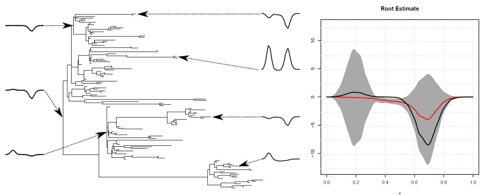
How might we reason about the forms of our unseen ancestors? I discuss a possible application to speech sounds in an earlier blog article (necrophonetics). A paper with John Moriarty which provides relevant theory came out lately in Royal Society Interface as "Evolutionary inference for function-valued traits: Gaussian process regression on phylogenies" (free version from this page). The gist of the idea is that some things in nature, like sounds or patterns, evolve in time and are best described as mathematical functions. Gaussian processes are a class of process which are very suited to the evolution of functions. An example of an evolving function would be a drawing of a line which is copied repeatedly (see here for a movie of us making school students do this). Having done the theory, Pantelis Hadjipantelis from Warwick (a student of John Aston) and  Chris Knight and David Springate helped take this further. They investigated whether our theory could be made to work in practice and considered careful simulated examples. In these we could see how our best estimate about characteristics of the evolutionary process and the form of the ancestors compared against (simulated) reality. We did reasonably well. On the way we used Independent Components Analysis - a very handy method. This work will be appearing shortly in Royal Society Interface as "Function-Valued Traits in Evolution" free version here. Having convinced ourselves of the relevance of the method for simulated data the next step was to consider real data that Chris Knight has - that paper is under-way. If this interests you then Mhairi Kerr produced a masters thesis on the topic working with Vincent Macaulay. This has some further introductory content. Nick

Functions can evolve along evolutionary trees - just like genetic sequences. On the left-hand we provide a simulation of function evolution. On the right we use the data from the leaves of the evolutionary tree to reconstruct the common ancestral function. Red line is the value of the function we expect/predict and black line is an actual value (in grey is a measure of our uncertainty)

Statistics vs Physics

While there's a whole branch of physics called statistical physics (probably a misleading title) physicists often get only a few hours of statistical training in their undergraduate degrees. This is surprising to some who think of physicists as the most mathematical of scientists. In fact you can find a diversity of statistical crimes/accidents in physics papers (and I'm sure you can find them in my own). In partial acknowledgement of this, I organised this Royal Society Discussion Meeting and edited this volume of the Philosophical Transactions of the Royal Society “Signal Processing and Inference for the Physical Sciences” with the excellent Prof Tom Maccarone (now at Texas Tech Astrophysics and Astronomy). Our goal was to expose physical scientists to some new topics in statistical inference and some data analysts to physical challenges. Lots of the volume is free and there are also talks from the authors and slides on this page. We provide an introduction "Inference for the Physical Sciences" which we hope can serve as a jumping off point for physical scientists wanting to use statistical tools. Max Little also wrote an article highlighting some challenges in signal processing in biophysics "Signal processing for molecular and cellular biological physics" putting some of our other work in context (see previous blog articles on finding steps beneath the noise and on molecular dance steps). For those with an interest in Machine Learning I think the talks by Bishop, Gharamani, Roberts and Hyvärinen are worth a look. Nick

Dr Ben Fulcher made the image above - similar signals are linked up (see a pending blog article) and we have to guess whether the green event that mysteriously occurred in Russia was a blue test explosion or a red earthquake...

Exploring noise in cellular biology

We're used to thinking about machines as robust, hard-wearing objects made from solid materials like metal and plastics. If they crack, split or overheat they are liable to malfunction, and if we subject them to too much jostling and shaking we're asking for trouble. However, the biochemical machines responsible for keeping us alive work in a rather different world -- they're made from soft, organic materials, and contained in a disorganised bag (the cell) that is constantly shaken, bumping our machines against each other and other cellular inhabitants. How can the delicate processes required by living organisms take place in this chaotic environment? And how can scientific progress be made in such a tumultuous, unpredictable world?

Extrinsic factors can modulate the stability of essential, but noisy, cellular circuits

Iain recently wrote an article, targeted at a broad audience, looking at some of these questions. One of the most important cellular processes that has to take place in this chaotic world is that of 'gene expression': the interpretation of genetic blueprints which describe how to build cellular machinery, and the subsequent construction process. Gene expression can be likened to using a bad photocopier to copy books from a library that opens and closes randomly, then using these photocopies (which are prone to decay) to construct machines. This problematic environment gives rise to many medically important random effects, including bacterial resistance to antibiotics and differing responses to anti-cancer drugs. We are particularly interested in how fluctuating power supplies (see our other blog articles here, here and here!) influence the cell's ability to produce these machines, and what effects this unreliable power has on medically important processes. The article -- available here and appearing in the expository magazine Significance -- takes a look at how cellular noise arises, current techniques for its detection and analysis, and its influence on important biological phenomena. Iain

Organizing networks using their dense regions

Many systems in fields ranging from biology to sociology, to politics and finance can be represented as networks. For example, in protein interaction networks each node represents a protein and each link, connecting a pair of nodes, quantifies the strength of the interaction between those proteins. Similarly, in political voting networks nodes represent politicians and the edges connecting pairs of politicians represent the similarity of their legislative voting records. Despite the significant differences in the underlying systems, the common network representation enables researchers in different fields to ask questions that can be surprisingly similar. Given this, it would be useful to have a systematic method to highlight similarities in networks from different fields to identify problems that might be tackled using the same techniques. For example, if a biological network representing covariation in neural activity in different regions of the brain could be shown to be structurally similar to a financial network representing correlation of stock returns, certain analytical tools and models might be applicable to both problems.

A taxonomy of networks

In our paper, we tackle this problem by first developing a method to quantify the similarity of different networks based on their community structure. A community in a network, loosely put, is a set of nodes which are more connected to each other than they are to the rest of the network (like a group of friends who have the majority of the social interactions with each-other). We introduce the idea of “mesoscopic response functions” which are curves that summarize the community structure of each network at different scales and enable us to define a single number that quantifies the similarity of network pairs. Importantly, this approach allows us to compare networks with different numbers of nodes and different link densities. We then use this similarity measure to construct taxonomies of networks. From an historical perspective, classification of objects in this way has been central to the progress of science, as demonstrated by the periodic table of elements in chemistry and the phylogenetic tree of organisms in biology.

The taxonomies constructed using our approach are successful at grouping networks that are known to be similar. For example, political voting networks for the US Congress, UK House of Commons and United Nation are clustered together in the same group. Perhaps more importantly, the method also identifies networks that are not grouped with members of the same class and are therefore unusual in some way. For example, a Facebook network for Caltech is not grouped with the Facebook networks of other universities. We also used the technique to detect historically significant financial and political changes in temporal sequences of networks; we found the stock market network corresponding to the 1987 crash and the voting network corresponding to the American Civil War to stand out from their respective sequences of networks.

You can read the full story in our paper “Taxonomies of networks from community structure” in Physical Review E 86, 036104 (2012)  In the paper, we demonstrate the range of fields in which this approach can be usefully applied using a set of 746 networks and case studies that include US Congressional voting, Facebook friendship, fungal growth, United Nations voting, and stock market return correlation networks. Dan, JP and Nick

How conserved are protein-protein interactions? And why would you want to know?

A comparison of biological sequences from multiple species shows a great deal of evolutionary conservation. An overall question of interest is the following: what is the connection between similarities in biological sequence between species and similarities in the function of their components and cells?

We started to think about this question in the specific context of proteins: the construction blocks of cells which are specified by a sequence (of amino acids). If two human proteins are known to physically interact (stick to each other) will their equivalent (homologous) proteins in mouse physically interact? (To say that two proteins are homologous means that they are similar through common evolutionary descent: in some sense, they are the 'same' protein).

The answer, it is often assumed, is 'yes': a fairly similar sequence that specifies the protein makes for a fairly similar function of that protein. Indeed, partly because new sequence data is being generated at a much faster rate than any other type of data, it is common practice to 'transfer' functional knowledge (such as interaction partners) from a functionally characterised protein to its unstudied matches in other species. But is this legitimate?

If we know the interaction between proteins in the network of the green organism what can we say about the  interactions of similar proteins in the blue organism's network?

An answer could also shed light on more theoretical questions.
- If only small changes in sequence can lead to new interactions between proteins, then this could be a fast evolutionary mechanism to generate new functions.
- Homologs are also found within a species - do these maintain the same interactions (a form of robustness), or rapidly lose them (release from evolutionary selection)?

Our paper just appeared in PLoS Computational Biology with the title "What Evidence is There for the Homology of Protein-Protein Interactions?". Our results returned some expected conclusions: more closely related species have more conserved interactions; the more stringent the definition to consider two proteins as homologs, the more conservation observed. An overall conclusion was that, at definitions of homology/similarity frequently used in the community, conservation of interactions is low, and hence 'transferred' functional annotations should be used with care. We also compared the transfer of interactions between and within species, and found within-species transfers were less reliable than between-species transfers. Using our method we also made some guesses as to the rate at which protein-protein interactions are lost through evolutionary time and about the total number of interactions that are present between all the proteins in an organism.

Our work is preliminary in many ways: better attempts at dealing with interaction data errors could be made; we treated all the interactions as independent of each other, which of course they are not; we didn't compare our derived rate of loss of interactions with other evolutionary rates; and much else besides! Hopefully someone else will pick up where we have left off... Anna and Nick

Predicting network flows

Many biological, geophysical and technological systems involve the transport of material over a network by bulk fluid flow (advection) and diffusion within that fluid. The analogy is that ink spilled in the middle of a river both spreads out symmetrically by diffusion (even if the river were stationary) and also gets transported bodily with the flow of the river (advection). Bulk fluid transport systems are found in the vast majority of multi-cellular organisms, as the component cells of such organisms require resources for metabolism and growth, and the speed of diffusion alone is often such that it is only an effective means of exchange at microscopic length scales.  Molecules of interest are carried by advection and diffusion through the networks that make up fungi, the blood vessel networks of animals, the xylem and phloem elements of plants, and various body cavities of many different animals. Advection and diffusion are also fundamental to transport in geological and technological systems, such as rivers and drainage networks, gas pipelines, sewer systems and ventilation systems.

In all of these cases the particles of interest diffuse within a moving fluid, which is constrained to flow within a given network. Furthermore, the molecules that are carried through the network may be consumed or delivered out of the network at a particular rate. For example, glucose molecules are carried through the blood, and at each point in the network there is some probability that a given glucose molecule will be transported out of the vascular system and into the surrounding tissue. We have recently developed an algorithm for predicting how the spatial distribution of nutrients in a network will vary over space and time, when the resource in question is subject to given rates of advection, diffusion and delivery. We explain the algorithm in our paper "Advection, diffusion, and delivery over a network" that recently appeared in Physical Review E. 

(a) Phanerochaete velutina in a 24cm x 24cm microcosm, photographed just before radio-tracer was dripped onto the inoculum.

(b) Data from the photon counting camera. The brightness of the image reflects the concentration of the tracer in each part of the network.

(c) Digitized network, coloured to indicate the tracer concentration. Concentration is measured in arbitrary units, and edges that could not be measured are coloured black.

(d) Predicted concentration measured in arbitrary units, under the assumption that the tracer enters the network at the inoculum at a constant rate, each edge in the final network continues to grow (or shrink) at the same rate that was observed over the final time step, and 10% of each edge is occupied by transport vessels.

(e) Predicted intensity in arbitrary units under the same assumptions as diagram d), except that in this case we assume that 20% of each edge is occupied by transport vessels.

We are particularly interested in modeling the movement of radio-labelled tracers in growing fungal networks. As mentioned in a previous post, we hypothesize that within fungal networks, there is a bulk movement of fluid from the sites of water uptake to the sites of growth. To test this hypothesis, we allowed the fungi Phanerochaete velutina to grow on a dish for a four week period, taking photographs every three days. An image analysis program was then used to convert the sequence of photographs into a sequence of networks, comprised of edges of measured length and volume.

After taking a final photograph of our fungi, we added a radio-labelled tracer, placed a scintillation screen over the network, and used a photon counting camera to see where the tracer moved. This experiment gave us empirical data which we could use to evaluate our model of transport in fungal networks. Our model has one free parameter, corresponding to the fraction of each edge that is occupied by transport vessels. We found that our model (see Fig. d) of growth-induced mass flows was remarkably good at predicting where the tracers would spread (compare to Fig c), if we make the biologically plausible assumption that the fluid flows occur within transport vessels that occupy 10% of each edge in the network. Luke and Nick 

Educated guesses about ancestral shapes and sounds: what do dead languages like Latin and Greek sound like?

What might ancient creatures have looked like? What would dead languages have sounded like? And what are the evolutionary relationships between currently observed shapes and sounds? While we have widely accepted methods that allow us to speculate (in an educated fashion) about ancestral genetic sequences we don't have well developed approaches for shapes and  functions.

I proposed to John Moriarty that we attempt to extend sequence inference to functions, and we got a grant with some most excellent colleagues John Aston, Dorothy Buck and Vincent Macaulay. John and I wrote a paper in which we investigated this using the versatile mathematical tools that are Gaussian Processes. We showed that in some controlled settings we could take (functional) observations from the world and make sensible guesses about what their ancestors might have been. If you want to see a video of us implementing an experiment with the help of some school children then click here (a blog specifically about our school engagement is here). More or less, our task is to take the game of telephone and run it backwards to identify the original sound (a sound can be viewed as a curve, or function on the line, or as, e.g., a spectrogram, a function on the plane).

But once you suppose you can reconstruct original sounds from mutated versions then one might hope to engage with some big and old questions: what do dead languages like Latin and Greek sound like? Can we use observations of contemporary speech sounds made at different leaves of linguistic trees (see the picture below) "to put probability distributions over" (make educated guesses about) possible ancestral speech sounds? One takes an audio recording of the same (sufficiently homologous) word in multiple different languages and attempts to make (probabilistic) inferences about the corresponding ancestral sounds.

On the left is Schleicher's original tree of Indo-European languages, from 1860. On the right is a numerical experiment where, given knowledge of the three black curves at the bottom and the evolutionary tree (thick black object) we can put a probability distribution over possible ancestral curves and sample from that distribution (red curve is the mean, blue a measure of standard deviation and dotted black is a sample from that distribution).

We just wrote a relatively non-technical paper in Trends in Ecology and Evolution "Phylogenetic inference for function-valued traits: speech sound evolution" (free version here and not free version here) with authors: John Aston (Warwick Stats) Dorothy Buck (Imperial Maths), John Coleman (Oxford Phonetics), Colin Cotter (Imperial Aero), NJ, Vincent Macaulay (Glasgow Stats), Norman Macleod (Natural History Museum), John Moriarty (Manchester Maths), Andrew Nevins (UCL Linguistics). In this we suggest that we have all the tools to try to reconstruct ancient speech (we also have lots of people with strong opinions about what ancient speech might have sounded like). We also use the paper to emphasise that this approach could allow us to reconstruct evolutionary trees from (functional) data. John Coleman says that they're (informally) calling this activity of reconstructing past speech sounds, necro-phonetics. I think that's neat. Nick